import numpy as np
import pandas as pd
import matplotlib.pyplot as plt
import seaborn as sns
from sklearn.datasets import make_hastie_10_2

sns.set_theme()

# HASTIE Data
X, Y = make_hastie_10_2(n_samples=4000, random_state=42)

df = pd.DataFrame(X)

df.columns = [f"{nmb}_NUM" for nmb in df.columns]

# add cat. features
df['1_CAT'] = ['cat1', 'cat2', 'cat1', 'cat2', 'cat1'] * (len(df) //  5)
df['2_CAT'] = ['catA', 'catB', 'catA', 'catB', 'catA'] * (len(df) //  5)

# Convert the new columns to categorical data
df['1_CAT'] = df['1_CAT'].astype('category')
df['2_CAT'] = df['2_CAT'].astype('category')

df["target"] = YSample Project for Binary Classification in high dimensions using Machine Learning Methods
Dieses Notebook soll das grundlegende Vorgehen eines Projekts zur binären Klassifizierung zusammenfassen.
Data Visualization and Descriptive Analysis
Generating a dummy dataset in style of of the unbalanced “real” dataset
df.groupby("target")["0_NUM"].count().plot.bar()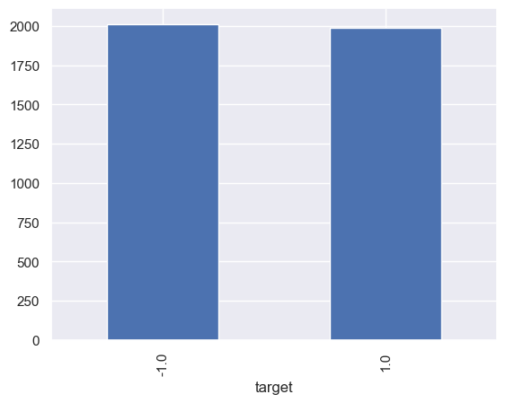
Now make this unbalanced
failed = df[df['target'] == -1]
num_rows_to_drop = int(len(failed) *  0.80)
rows_to_drop = failed.sample(n=num_rows_to_drop)
indices_to_drop = rows_to_drop.index

df = df.drop(indices_to_drop)

df.reset_index(drop=True, inplace=True)
df.groupby("target")["0_NUM"].count().plot.bar()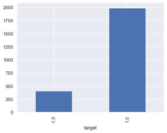
df.head()| 0_NUM | 1_NUM | 2_NUM | 3_NUM | 4_NUM | 5_NUM | 6_NUM | 7_NUM | 8_NUM | 9_NUM | 1_CAT | 2_CAT | target | |
|---|---|---|---|---|---|---|---|---|---|---|---|---|---|
| 0 | -0.463418 | -0.465730 | 0.241962 | -1.913280 | -1.724918 | -0.562288 | -1.012831 | 0.314247 | -0.908024 | -1.412304 | cat2 | catB | 1.0 |
| 1 | -0.601707 | 1.852278 | -0.013497 | -1.057711 | 0.822545 | -1.220844 | 0.208864 | -1.959670 | -1.328186 | 0.196861 | cat2 | catB | 1.0 |
| 2 | 0.738467 | 0.171368 | -0.115648 | -0.301104 | -1.478522 | -0.719844 | -0.460639 | 1.057122 | 0.343618 | -1.763040 | cat1 | catA | -1.0 |
| 3 | -0.479174 | -0.185659 | -1.106335 | -1.196207 | 0.812526 | 1.356240 | -0.072010 | 1.003533 | 0.361636 | -0.645120 | cat2 | catB | -1.0 |
| 4 | 0.361396 | 1.538037 | -0.035826 | 1.564644 | -2.619745 | 0.821903 | 0.087047 | -0.299007 | 0.091761 | -1.987569 | cat1 | catA | 1.0 |
df.describe()| 0_NUM | 1_NUM | 2_NUM | 3_NUM | 4_NUM | 5_NUM | 6_NUM | 7_NUM | 8_NUM | 9_NUM | target | |
|---|---|---|---|---|---|---|---|---|---|---|---|
| count | 2391.000000 | 2391.000000 | 2391.000000 | 2391.000000 | 2391.000000 | 2391.000000 | 2391.000000 | 2391.000000 | 2391.000000 | 2391.000000 | 2391.000000 |
| mean | -0.022469 | 0.013597 | -0.014034 | -0.018952 | -0.024258 | -0.024186 | 0.032337 | 0.009684 | -0.006151 | 0.013522 | 0.662903 |
| std | 1.144197 | 1.097748 | 1.108117 | 1.090767 | 1.113106 | 1.112722 | 1.114094 | 1.130735 | 1.100124 | 1.059689 | 0.748862 |
| min | -3.922400 | -4.465604 | -3.635200 | -3.367806 | -3.856375 | -3.232565 | -3.448043 | -3.601085 | -3.307900 | -3.176704 | -1.000000 |
| 25% | -0.818183 | -0.743014 | -0.805686 | -0.780403 | -0.792145 | -0.809809 | -0.715944 | -0.785525 | -0.753489 | -0.698564 | 1.000000 |
| 50% | -0.025494 | -0.011878 | -0.005658 | -0.037915 | -0.034257 | -0.008790 | 0.030849 | 0.011996 | 0.005458 | 0.008556 | 1.000000 |
| 75% | 0.806072 | 0.752285 | 0.758793 | 0.739861 | 0.755324 | 0.748119 | 0.786833 | 0.789278 | 0.742089 | 0.758722 | 1.000000 |
| max | 3.727833 | 3.942331 | 3.691625 | 4.479084 | 3.287761 | 3.926238 | 3.602832 | 3.335268 | 3.377768 | 3.852731 | 1.000000 |
Define Features \(X\) and Target \(Y\)
features = list(df.columns)
cat_features = ["1_CAT", "2_CAT"]
num_features = [feat for feat in features if feat not in["target", *cat_features]]
target = "target"
Main Part
Ab hier sollte dieses Notebook immer funktionieren, solange ein pandas DataFrame df, ein Liste numerischer Features num_features, eine Liste kategorialer Features cat_features sowie eine String-Variable target vorher definiert wurde.
Alles hier drunter dann einfach durchlaufen lassen 👩
Plot \(X_i \sim X_j\) for all \(i \ne j\) for \(X \in \mathbb{R}^p\) and \(i, \, j = \{1, \, \dots, \, p\}\). and color points / distributions by the target class \(Y \in \{0, \, 1\}\).
sns.pairplot(data=df,
             y_vars=num_features,
             x_vars=num_features,
             hue="target")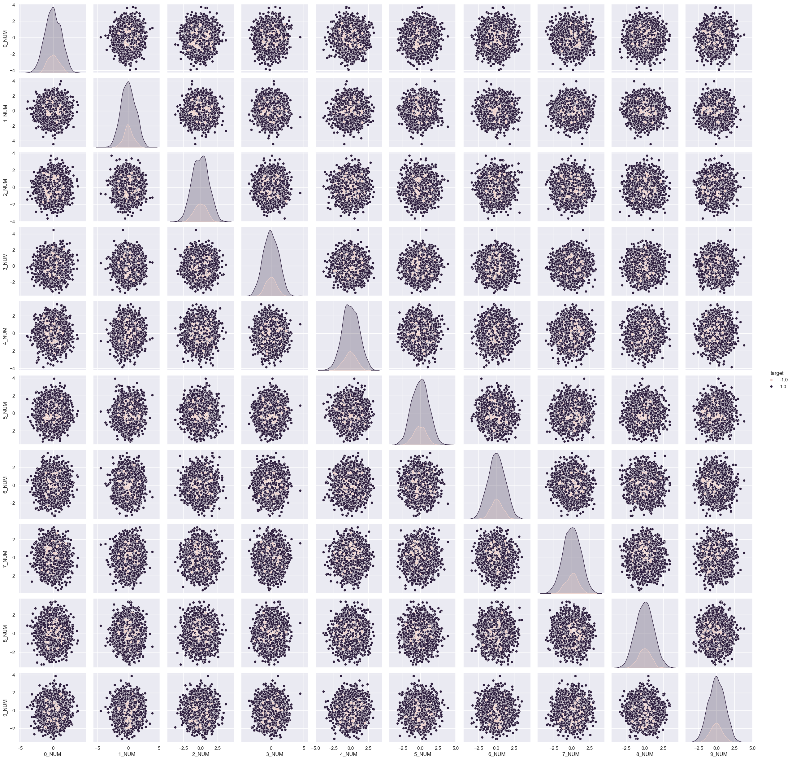
sns.catplot(data=df, x=cat_features[1], y=target)
Split to features and target
X = df[[*num_features, *cat_features]].to_numpy()
Y = df[target].to_numpy()

X_df = df[[*num_features, *cat_features]]
Y_df = df[target]
First Classification Approaches
Prepare Data: Train / Test split, min / max thresholds
# Prepare Data for Evaluating Learners
from sklearn.model_selection import train_test_split

X_train, X_test, y_train, y_test = train_test_split(
        X_df, Y_df, test_size=0.25, random_state=42, stratify=Y_df
    )

x_min, x_max = X[:, 0].min() - 0.5, X[:, 0].max() + 0.5
y_min, y_max = X[:, 1].min() - 0.5, X[:, 1].max() + 0.5

# Prepare Colours
from matplotlib.colors import ListedColormap

cm = plt.cm.RdBu
cm_bright = ListedColormap(["#FF0000", "#0000FF"])
Define Classifiers to compare
from sklearn.discriminant_analysis import QuadraticDiscriminantAnalysis
from sklearn.ensemble import AdaBoostClassifier, RandomForestClassifier
from sklearn.gaussian_process import GaussianProcessClassifier
from sklearn.gaussian_process.kernels import RBF
from sklearn.inspection import DecisionBoundaryDisplay
from sklearn.model_selection import train_test_split
from sklearn.naive_bayes import GaussianNB
from sklearn.neighbors import KNeighborsClassifier
from sklearn.neural_network import MLPClassifier
from sklearn.svm import SVC
from sklearn.tree import DecisionTreeClassifier
from sklearn.dummy import DummyClassifier
from sklearn.linear_model import LogisticRegressionCV

from sklearn.preprocessing import StandardScaler, OneHotEncoder
from sklearn.compose import ColumnTransformer

names = [
    "Baseline Dummy",
    "LogisticRegression",
    "LassoClassifier",
    "RidgeClassifier",
    "Nearest Neighbors",
    "Linear SVM",
    "RBF SVM",
    "Gaussian Process",
    "Decision Tree",
    "Random Forest",
    "Neural Net",
    "AdaBoost",
    "Naive Bayes",
    "QDA",
]


classifiers = [
    DummyClassifier(strategy="most_frequent"),
    LogisticRegressionCV(),
    LogisticRegressionCV(penalty="l1", solver="liblinear"),
    LogisticRegressionCV(penalty="l2"),
    KNeighborsClassifier(3),
    SVC(kernel="linear", C=0.025, random_state=42),
    SVC(gamma=2, C=1, random_state=42),
    GaussianProcessClassifier(1.0 * RBF(1.0), random_state=42),
    DecisionTreeClassifier(max_depth=5, random_state=42),
    RandomForestClassifier(
        max_depth=5, n_estimators=10, max_features=1, random_state=42
    ),
    MLPClassifier(alpha=1, max_iter=1000, random_state=42),
    AdaBoostClassifier(algorithm="SAMME", random_state=42),
    GaussianNB(),
    QuadraticDiscriminantAnalysis(),
]


preprocessor = ColumnTransformer(
    transformers=[
        ('num', StandardScaler(), num_features),
        ('cat', OneHotEncoder(), cat_features)
    ])
from sklearn.metrics import classification_report
from sklearn.metrics import RocCurveDisplay
from sklearn.metrics import PrecisionRecallDisplay
from sklearn.pipeline import Pipeline
n_classifiers = len(classifiers)
scaling = 8
fig, axes = plt.subplots(nrows=n_classifiers, ncols=2, figsize=(scaling, int(0.5*n_classifiers*scaling)))
reports_base = {}
for idx, (name, clf) in enumerate(zip(names, classifiers)):
clf = Pipeline(steps=[("preprocessor", preprocessor), ("clf", clf)])
clf.fit(X_train, y_train)
y_pred = clf.predict(X_test)
print(f"\n\n\n Report of {name}:\n {classification_report(y_test, y_pred, zero_division=0)}")
# Create ROC curve display
roc_display = RocCurveDisplay.from_estimator(clf, X_test, y_test, name=name, ax=axes[idx, 0])
axes[idx, 0].set_title(f"ROC Curve for {name}\n(over test sample)")
# Create Precision-Recall curve display
pr_display = PrecisionRecallDisplay.from_estimator(clf, X_test, y_test, name=name, ax=axes[idx, 1])
axes[idx, 1].set_title(f"Precision-Recall Curve for {name}\n(over test sample)")
# Store classification report
reports_base[name] = classification_report(y_test, y_pred, zero_division=0, output_dict=True)
plt.subplots_adjust(hspace=0.5, wspace=0.5)
plt.tight_layout()
fig.tight_layout()
plt.show()
 Report of Baseline Dummy:
               precision    recall  f1-score   support

        -1.0       0.00      0.00      0.00       101
         1.0       0.83      1.00      0.91       497

    accuracy                           0.83       598
   macro avg       0.42      0.50      0.45       598
weighted avg       0.69      0.83      0.75       598


 Report of LogisticRegression:
               precision    recall  f1-score   support

        -1.0       0.00      0.00      0.00       101
         1.0       0.83      1.00      0.91       497

    accuracy                           0.83       598
   macro avg       0.42      0.50      0.45       598
weighted avg       0.69      0.83      0.75       598


 Report of LassoClassifier:
               precision    recall  f1-score   support

        -1.0       0.00      0.00      0.00       101
         1.0       0.83      1.00      0.91       497

    accuracy                           0.83       598
   macro avg       0.42      0.50      0.45       598
weighted avg       0.69      0.83      0.75       598


 Report of RidgeClassifier:
               precision    recall  f1-score   support

        -1.0       0.00      0.00      0.00       101
         1.0       0.83      1.00      0.91       497

    accuracy                           0.83       598
   macro avg       0.42      0.50      0.45       598
weighted avg       0.69      0.83      0.75       598


 Report of Nearest Neighbors:
               precision    recall  f1-score   support

        -1.0       0.41      0.67      0.51       101
         1.0       0.92      0.80      0.86       497

    accuracy                           0.78       598
   macro avg       0.67      0.74      0.69       598
weighted avg       0.84      0.78      0.80       598


 Report of Linear SVM:
               precision    recall  f1-score   support

        -1.0       0.00      0.00      0.00       101
         1.0       0.83      1.00      0.91       497

    accuracy                           0.83       598
   macro avg       0.42      0.50      0.45       598
weighted avg       0.69      0.83      0.75       598


 Report of RBF SVM:
               precision    recall  f1-score   support

        -1.0       0.00      0.00      0.00       101
         1.0       0.83      1.00      0.91       497

    accuracy                           0.83       598
   macro avg       0.42      0.50      0.45       598
weighted avg       0.69      0.83      0.75       598


 Report of Gaussian Process:
               precision    recall  f1-score   support

        -1.0       0.00      0.00      0.00       101
         1.0       0.83      1.00      0.91       497

    accuracy                           0.83       598
   macro avg       0.42      0.50      0.45       598
weighted avg       0.69      0.83      0.75       598


 Report of Decision Tree:
               precision    recall  f1-score   support

        -1.0       0.00      0.00      0.00       101
         1.0       0.83      0.99      0.90       497

    accuracy                           0.82       598
   macro avg       0.41      0.49      0.45       598
weighted avg       0.69      0.82      0.75       598


 Report of Random Forest:
               precision    recall  f1-score   support

        -1.0       0.00      0.00      0.00       101
         1.0       0.83      1.00      0.91       497

    accuracy                           0.83       598
   macro avg       0.42      0.50      0.45       598
weighted avg       0.69      0.83      0.75       598


 Report of Neural Net:
               precision    recall  f1-score   support

        -1.0       0.96      0.47      0.63       101
         1.0       0.90      1.00      0.95       497

    accuracy                           0.91       598
   macro avg       0.93      0.73      0.79       598
weighted avg       0.91      0.91      0.89       598


 Report of AdaBoost:
               precision    recall  f1-score   support

        -1.0       0.00      0.00      0.00       101
         1.0       0.83      1.00      0.91       497

    accuracy                           0.83       598
   macro avg       0.42      0.50      0.45       598
weighted avg       0.69      0.83      0.75       598


 Report of Naive Bayes:
               precision    recall  f1-score   support

        -1.0       1.00      0.25      0.40       101
         1.0       0.87      1.00      0.93       497

    accuracy                           0.87       598
   macro avg       0.93      0.62      0.66       598
weighted avg       0.89      0.87      0.84       598


 Report of QDA:
               precision    recall  f1-score   support

        -1.0       0.22      0.58      0.32       101
         1.0       0.87      0.58      0.70       497

    accuracy                           0.58       598
   macro avg       0.55      0.58      0.51       598
weighted avg       0.76      0.58      0.63       598
c:\ProgramData\anaconda3\envs\quarto_dev\Lib\site-packages\sklearn\discriminant_analysis.py:935: UserWarning: Variables are collinear
  warnings.warn("Variables are collinear")
reform_base = {(learner, class_label): values for learner, innerDict in reports_base.items() for class_label, values in innerDict.items()}
reports_base_df = pd.DataFrame(reform_base).T
ax = reports_base_df.loc[:, "f1-score"].loc[:, "weighted avg"].plot.bar(title="F1-Score (weighted avg.) for base models \n (without tuning, without variable selection, without dim-reduction)",
figsize=(12,8))
ax.bar_label(ax.containers[0], padding=1, fmt="%.3f")[Text(0, 1, '0.754'),
Text(0, 1, '0.754'),
Text(0, 1, '0.754'),
Text(0, 1, '0.754'),
Text(0, 1, '0.801'),
Text(0, 1, '0.754'),
Text(0, 1, '0.754'),
Text(0, 1, '0.754'),
Text(0, 1, '0.750'),
Text(0, 1, '0.754'),
Text(0, 1, '0.892'),
Text(0, 1, '0.754'),
Text(0, 1, '0.839'),
Text(0, 1, '0.633')]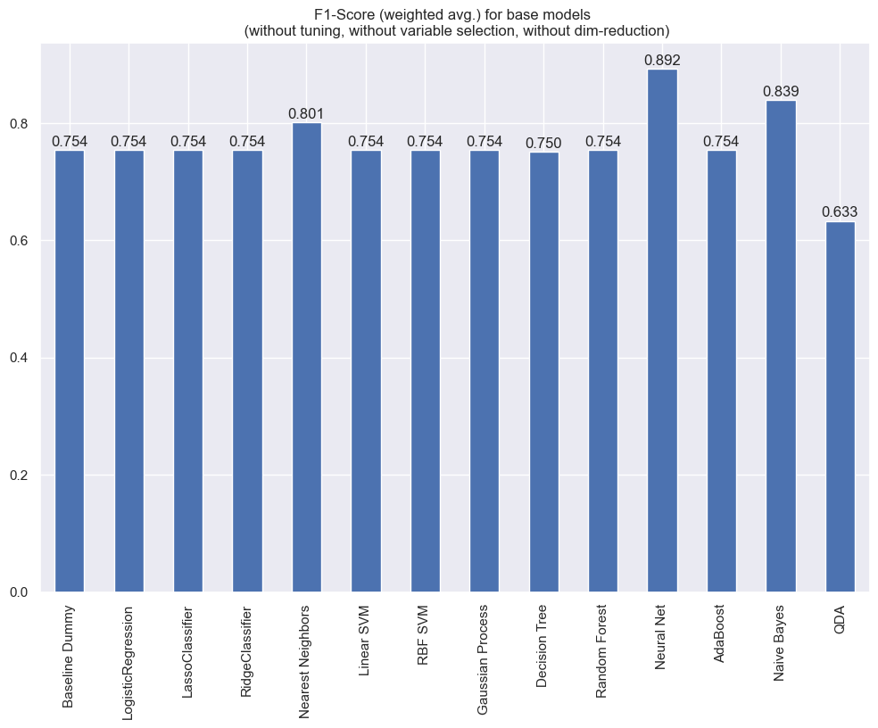
ax = reports_base_df.loc[:, "f1-score"].loc[:, "accuracy"].plot.bar(title="Accuracy (weighted avg.) for base models \n (without tuning, without variable selection, without dim-reduction)",
                                                               figsize=(12,8))
ax.bar_label(ax.containers[0], padding=1, fmt="%.3f")
[Text(0, 1, '0.831'),
Text(0, 1, '0.831'),
Text(0, 1, '0.831'),
Text(0, 1, '0.831'),
Text(0, 1, '0.783'),
Text(0, 1, '0.831'),
Text(0, 1, '0.831'),
Text(0, 1, '0.831'),
Text(0, 1, '0.823'),
Text(0, 1, '0.831'),
Text(0, 1, '0.906'),
Text(0, 1, '0.831'),
Text(0, 1, '0.873'),
Text(0, 1, '0.580')]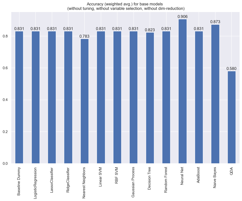
Add methods to handle unbalanced dataset
Using Synthetic Minority Oversampling Technique (SMOTE)
from imblearn.over_sampling import SMOTE

smt = SMOTE(random_state=42)
from sklearn.metrics import classification_report
from sklearn.metrics import RocCurveDisplay
from sklearn.metrics import PrecisionRecallDisplay
from imblearn.pipeline import Pipeline as imb_Pipeline
n_classifiers = len(classifiers)
scaling = 8
fig, axes = plt.subplots(nrows=n_classifiers, ncols=2, figsize=( scaling, int(0.5*n_classifiers*scaling)))
reports_smote = {}
for idx, (name, clf) in enumerate(zip(names, classifiers)):
clf = imb_Pipeline(steps=[("preprocessor", preprocessor), ('smote', smt), ("clf", clf)])
clf.fit(X_train, y_train)
y_pred = clf.predict(X_test)
print(f"\n\n\n Report of {name}:\n {classification_report(y_test, y_pred, zero_division=0)}")
# Create ROC curve display
roc_display = RocCurveDisplay.from_estimator(clf, X_test, y_test, name=name, ax=axes[idx, 0])
axes[idx, 0].set_title(f"ROC Curve for {name}\n(over test sample)")
# Create Precision-Recall curve display
pr_display = PrecisionRecallDisplay.from_estimator(clf, X_test, y_test, name=name, ax=axes[idx, 1])
axes[idx, 1].set_title(f"Precision-Recall Curve for {name}\n(over test sample)")
# Store classification report
reports_smote[name] = classification_report(y_test, y_pred, zero_division=0, output_dict=True)
plt.subplots_adjust(hspace=0.5, wspace=0.5)
plt.tight_layout()
fig.tight_layout()
plt.show()
 Report of Baseline Dummy:
               precision    recall  f1-score   support

        -1.0       0.17      1.00      0.29       101
         1.0       0.00      0.00      0.00       497

    accuracy                           0.17       598
   macro avg       0.08      0.50      0.14       598
weighted avg       0.03      0.17      0.05       598


 Report of LogisticRegression:
               precision    recall  f1-score   support

        -1.0       0.16      0.47      0.24       101
         1.0       0.82      0.50      0.62       497

    accuracy                           0.49       598
   macro avg       0.49      0.48      0.43       598
weighted avg       0.71      0.49      0.56       598


 Report of LassoClassifier:
               precision    recall  f1-score   support

        -1.0       0.15      0.43      0.22       101
         1.0       0.81      0.51      0.62       497

    accuracy                           0.49       598
   macro avg       0.48      0.47      0.42       598
weighted avg       0.70      0.49      0.56       598


 Report of RidgeClassifier:
               precision    recall  f1-score   support

        -1.0       0.16      0.47      0.24       101
         1.0       0.82      0.50      0.62       497

    accuracy                           0.49       598
   macro avg       0.49      0.48      0.43       598
weighted avg       0.71      0.49      0.56       598


 Report of Nearest Neighbors:
               precision    recall  f1-score   support

        -1.0       0.27      0.85      0.41       101
         1.0       0.95      0.54      0.69       497

    accuracy                           0.59       598
   macro avg       0.61      0.70      0.55       598
weighted avg       0.83      0.59      0.64       598


 Report of Linear SVM:
               precision    recall  f1-score   support

        -1.0       0.15      0.48      0.23       101
         1.0       0.81      0.45      0.58       497

    accuracy                           0.45       598
   macro avg       0.48      0.46      0.40       598
weighted avg       0.70      0.45      0.52       598


 Report of RBF SVM:
               precision    recall  f1-score   support

        -1.0       0.00      0.00      0.00       101
         1.0       0.83      1.00      0.91       497

    accuracy                           0.83       598
   macro avg       0.42      0.50      0.45       598
weighted avg       0.69      0.83      0.75       598
c:\ProgramData\anaconda3\envs\quarto_dev\Lib\site-packages\sklearn\gaussian_process\kernels.py:434: ConvergenceWarning: The optimal value found for dimension 0 of parameter k1__constant_value is close to the specified upper bound 100000.0. Increasing the bound and calling fit again may find a better value.
  warnings.warn(
 Report of Gaussian Process:
               precision    recall  f1-score   support

        -1.0       0.98      0.89      0.93       101
         1.0       0.98      1.00      0.99       497

    accuracy                           0.98       598
   macro avg       0.98      0.94      0.96       598
weighted avg       0.98      0.98      0.98       598


 Report of Decision Tree:
               precision    recall  f1-score   support

        -1.0       0.23      0.69      0.34       101
         1.0       0.89      0.53      0.66       497

    accuracy                           0.56       598
   macro avg       0.56      0.61      0.50       598
weighted avg       0.78      0.56      0.61       598


 Report of Random Forest:
               precision    recall  f1-score   support

        -1.0       0.35      0.72      0.47       101
         1.0       0.93      0.72      0.81       497

    accuracy                           0.72       598
   macro avg       0.64      0.72      0.64       598
weighted avg       0.83      0.72      0.75       598


 Report of Neural Net:
               precision    recall  f1-score   support

        -1.0       0.90      0.73      0.81       101
         1.0       0.95      0.98      0.97       497

    accuracy                           0.94       598
   macro avg       0.93      0.86      0.89       598
weighted avg       0.94      0.94      0.94       598


 Report of AdaBoost:
               precision    recall  f1-score   support

        -1.0       0.38      0.81      0.52       101
         1.0       0.95      0.73      0.82       497

    accuracy                           0.74       598
   macro avg       0.66      0.77      0.67       598
weighted avg       0.85      0.74      0.77       598


 Report of Naive Bayes:
               precision    recall  f1-score   support

        -1.0       0.90      0.74      0.82       101
         1.0       0.95      0.98      0.97       497

    accuracy                           0.94       598
   macro avg       0.93      0.86      0.89       598
weighted avg       0.94      0.94      0.94       598


 Report of QDA:
               precision    recall  f1-score   support

        -1.0       0.26      0.84      0.40       101
         1.0       0.94      0.51      0.66       497

    accuracy                           0.57       598
   macro avg       0.60      0.68      0.53       598
weighted avg       0.83      0.57      0.62       598
c:\ProgramData\anaconda3\envs\quarto_dev\Lib\site-packages\sklearn\discriminant_analysis.py:935: UserWarning: Variables are collinear
  warnings.warn("Variables are collinear")
reform_smote = {(learner, class_label): values for learner, innerDict in reports_smote.items() for class_label, values in innerDict.items()}
reports_smote_df = pd.DataFrame(reform_smote).T
ax = reports_smote_df.loc[:, "f1-score"].loc[:, "weighted avg"].plot.bar(title="F1-Score (weighted avg.) for SMOTE models \n (without tuning, without variable selection, without dim-reduction)",
figsize=(12,8))
ax.bar_label(ax.containers[0], padding=1, fmt="%.3f")[Text(0, 1, '0.049'),
Text(0, 1, '0.557'),
Text(0, 1, '0.556'),
Text(0, 1, '0.557'),
Text(0, 1, '0.641'),
Text(0, 1, '0.518'),
Text(0, 1, '0.754'),
Text(0, 1, '0.978'),
Text(0, 1, '0.610'),
Text(0, 1, '0.754'),
Text(0, 1, '0.939'),
Text(0, 1, '0.772'),
Text(0, 1, '0.941'),
Text(0, 1, '0.617')]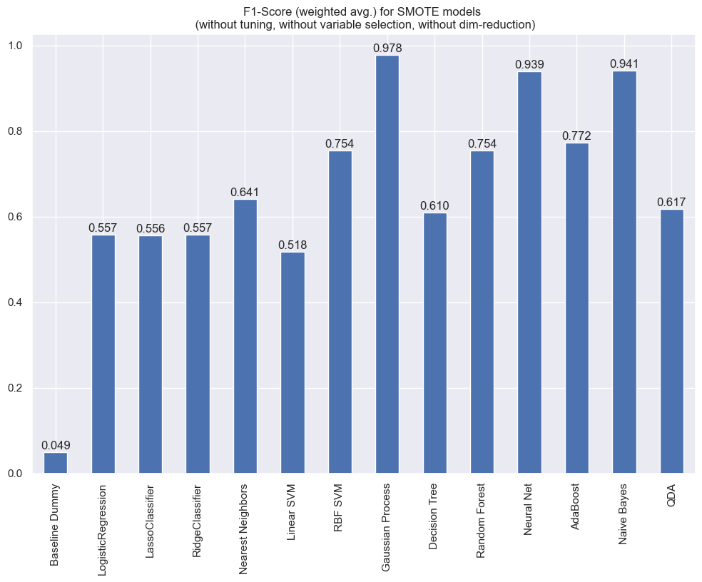
ax = reports_smote_df.loc[:, "f1-score"].loc[:, "accuracy"].plot.bar(title="Accuracy (weighted avg.) for SMOTE models \n (without tuning, without variable selection, without dim-reduction)",
                                                                     figsize=(12,8))
ax.bar_label(ax.containers[0], padding=1, fmt="%.3f")
[Text(0, 1, '0.169'),
Text(0, 1, '0.495'),
Text(0, 1, '0.493'),
Text(0, 1, '0.495'),
Text(0, 1, '0.592'),
Text(0, 1, '0.453'),
Text(0, 1, '0.831'),
Text(0, 1, '0.978'),
Text(0, 1, '0.555'),
Text(0, 1, '0.722'),
Text(0, 1, '0.941'),
Text(0, 1, '0.742'),
Text(0, 1, '0.943'),
Text(0, 1, '0.567')]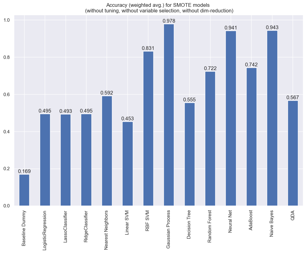
Dimensionality Reduction
PCA with linear Learner (LogReg)
from sklearn.decomposition import PCA
from sklearn.linear_model import LogisticRegression
from sklearn.model_selection import GridSearchCV
from sklearn.pipeline import Pipeline
from sklearn.preprocessing import StandardScaler

scaler = StandardScaler()
pca = PCA()
smt = SMOTE()

logistic = LogisticRegression(max_iter=10000)
# Define Pipeline
pca_pipe = imb_Pipeline(steps=[("preprocessor", preprocessor), ("smote", smt), ("pca", pca), ("logistic", logistic)])
# Fit PCA pipe
pca_param_grid = {
"pca__n_components": [n for n in range(1, 10)],
"logistic__C": np.logspace(-4, 4, 4),
}
pca_search = GridSearchCV(pca_pipe, pca_param_grid, n_jobs=2, scoring="f1")
pca_search.fit(X_train, y_train)
print("Best parameter (CV score=%0.3f):" % pca_search.best_score_)
print(pca_search.best_params_)Best parameter (CV score=0.671):
{'logistic__C': 10000.0, 'pca__n_components': 2}# Plot the PCA spectrum of Validation
pca.fit(preprocessor.transform(X_test))
fig, (ax0, ax1) = plt.subplots(nrows=2, sharex=True, figsize=(6, 6))
ax0.plot(
np.arange(1, pca.n_components_ + 1), pca.explained_variance_ratio_, "+", linewidth=2
)
ax0.set_ylabel("PCA explained variance ratio")
ax0.axvline(
pca_search.best_estimator_.named_steps["pca"].n_components,
linestyle=":",
label="n_components chosen",
)
ax0.legend(prop=dict(size=12))
# For each number of components, find the best classifier results
results = pd.DataFrame(pca_search.cv_results_)
components_col = "param_pca__n_components"
best_clfs = results.groupby(components_col)[
[components_col, "mean_test_score", "std_test_score"]
].apply(lambda g: g.nlargest(1, "mean_test_score"))
ax1.errorbar(
best_clfs[components_col],
best_clfs["mean_test_score"],
yerr=best_clfs["std_test_score"],
)
ax1.set_ylabel("Classification accuracy (val)")
ax1.set_xlabel("n_components")
plt.xlim(-1, len(features))
plt.tight_layout()
plt.show()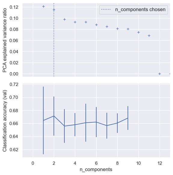
PCA with GPC
from sklearn.gaussian_process.kernels import DotProduct, RBF

pca = PCA()
smt = SMOTE()
gpc = GaussianProcessClassifier()

gpc_pipe = imb_Pipeline(steps=[("preprocessor", preprocessor), ("smote", smt), ("gpc", gpc)])

param_grid = {
    "gpc__kernel": [1.0 * RBF([1.0]), 1.0 * RBF([10.0])],
}
gpc_search = GridSearchCV(gpc_pipe, param_grid, n_jobs=-1, verbose=100, cv=3, scoring="f1")
gpc_search.fit(X_train, y_train)
print("Best parameter (CV score=%0.3f):" % gpc_search.best_score_)
print(gpc_search.best_params_)
y_pred = gpc_search.predict(X_test)
print(f"Report of GPC Pipe:\n {classification_report(y_test, y_pred)}")
# Create ROC curve display
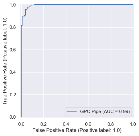
roc_display = RocCurveDisplay.from_estimator(gpc_search, X_test, y_test, name='GPC Pipe')
# Create Precision-Recall curve display
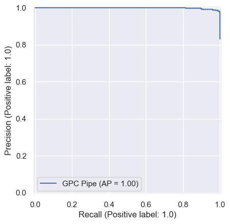
pr_display = PrecisionRecallDisplay.from_estimator(gpc_search, X_test, y_test, name='GPC Pipe')Fitting 3 folds for each of 2 candidates, totalling 6 fitsc:\ProgramData\anaconda3\envs\quarto_dev\Lib\site-packages\sklearn\gaussian_process\kernels.py:434: ConvergenceWarning: The optimal value found for dimension 0 of parameter k1__constant_value is close to the specified upper bound 100000.0. Increasing the bound and calling fit again may find a better value.
warnings.warn(Best parameter (CV score=0.987):
{'gpc__kernel': 1**2 * RBF(length_scale=1)}
Report of GPC Pipe:
precision recall f1-score support
-1.0 0.99 0.88 0.93 101
1.0 0.98 1.00 0.99 497
accuracy 0.98 598
macro avg 0.98 0.94 0.96 598
weighted avg 0.98 0.98 0.98 598
Sample Project for Binary Classification with Time Series as Features \(X\)
Generating synthetic data
Let \(X_1\), \(X_2\) be synthetic variables generated through the following DGP:
\[ X_1 := \alpha_0 + \beta_0 \sqrt{t} + \varepsilon_0, \quad \varepsilon_0 \sim \mathbb{N}(0, \sigma_0) \\ X_2 := \alpha_1 + \beta_1 \ln(t+1) + \zeta_1 \sin(t) + \varphi \frac{e^{-(t - \frac{n_{obs}}{2})^2}}{2 (\frac{\sigma_1}{2})^2} + \varepsilon_1, \quad \varepsilon_1 \sim \mathbb{N}(0, \sigma_1) \]
The output \(Y \in \{0,1\}\) is defined as
\[ Y := \begin{cases} &1 & \text{if } \max\{X_1\} + \frac{2}{T} \sum_{t \in T} X_2 < \theta \\ &-1 & \text{else} \end{cases} \]
num_timesteps = 800 # Number of time steps in each series
alpha = [0.4, 3.5] # Intercept
beta = [0.5, 1.3] # Slope
zeta_2 = 2
phi = 5
sigma = [1.6, 1.4] # Standard deviation of the noise

t = np.arange(num_timesteps)

x_1 = alpha[0] + beta[0] * np.sqrt(t) + np.random.normal(0, sigma[0], num_timesteps)
x_2 = alpha[1] + beta[1] * np.log(t+1) + zeta_2 * np.sin(t)  + phi * np.exp(-(t - num_timesteps/2)**2 / (2 * (sigma[1] / 2)**2)) + np.random.normal(0, sigma[1], num_timesteps)
sns.lineplot([x_1, x_2])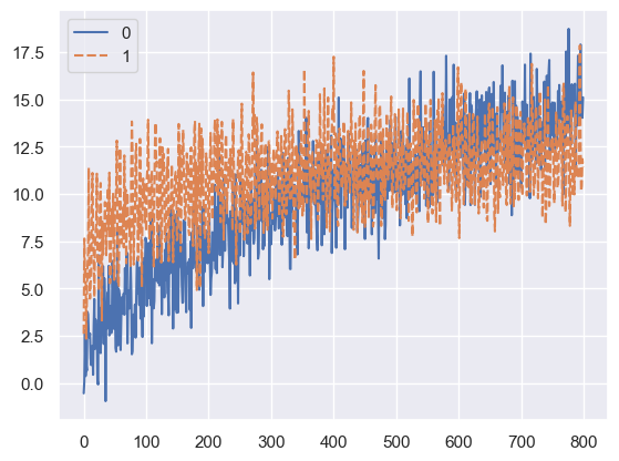
n_obs = 2600

theta = 40.5

time_series = []
binary_output = []

t = np.arange(num_timesteps)

X_ts = np.zeros((n_obs, 2, num_timesteps))
Y_ts = np.zeros(n_obs, )

np.random.seed(42)

for obs in range(n_obs): # Generate n_obs observations
  X_ts[obs, 0, :] = alpha[0] + beta[0] * np.sqrt(t) + np.random.normal(0, sigma[0], num_timesteps)
  X_ts[obs, 1, :] = alpha[1] + beta[1] * np.log(t+1) + zeta_2 * np.sin(t) + phi * np.exp(-(t - num_timesteps/2)**2 / (2 * (sigma[1] / 2)**2)) + np.random.normal(0, sigma[1], num_timesteps)
Y_ts[obs] = np.where(X_ts[obs, 0, :].max() + 2 * X_ts[obs, 1, :].mean() < theta, 1, -1)X_ts.shape(260, 2, 800)pd.DataFrame(Y_ts).groupby(by=0)[0].count().plot.bar()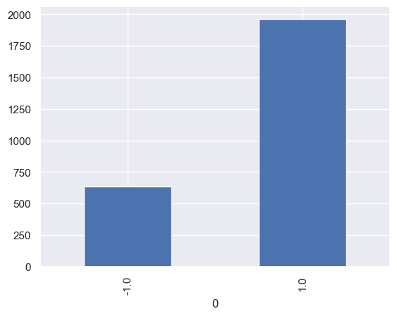
from sklearn.ensemble import RandomForestClassifier
from sklearn.model_selection import train_test_split
from sklearn.metrics import accuracy_score

from sktime.transformations.panel.tsfresh import TSFreshFeatureExtractor
from sktime.pipeline import make_pipeline

X_train, X_test, y_train, y_test = train_test_split(X_ts, Y_ts, test_size=0.25, random_state=42)

tsfresh_trafo = TSFreshFeatureExtractor(default_fc_parameters="minimal") #change to efficient for real analysis
clf = make_pipeline(tsfresh_trafo, RandomForestClassifier(n_estimators=100))
clf.fit(X_train, y_train)

y_pred = clf.predict(X_test)
Feature Extraction: 100%|██████████| 3900/3900 [00:02<00:00, 1510.88it/s]
Feature Extraction: 100%|██████████| 1300/1300 [00:00<00:00, 1452.65it/s]print(f"Report:\n {classification_report(y_test, y_pred)}")
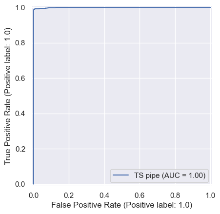
roc_display = RocCurveDisplay.from_estimator(clf, X_test, y_test, name='TS pipe')
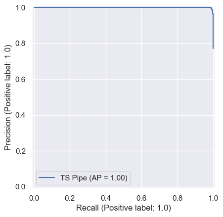
pr_display = PrecisionRecallDisplay.from_estimator(clf, X_test, y_test, name='TS Pipe')Report:
precision recall f1-score support
-1.0 0.97 0.97 0.97 149
1.0 0.99 0.99 0.99 501
accuracy 0.99 650
macro avg 0.98 0.98 0.98 650
weighted avg 0.99 0.99 0.99 650
Feature Extraction: 100%|██████████| 1300/1300 [00:00<00:00, 1820.93it/s]
Feature Extraction: 100%|██████████| 1300/1300 [00:01<00:00, 1160.08it/s]